section 4.2

section 4.2 The Definite Integral

Welcome to integral calculus!

Definition - the connection to area

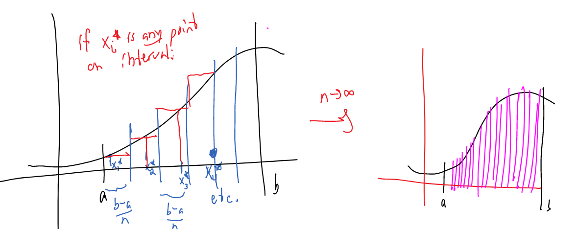
We define the definite integral of a function $f(x)$ on an interval $[a, b]$ by the following limit:

$$ \int_a^b f(x) \, dx = \lim_{n\to \infty} \sum_{i=1}^n f(x_i^*) \, \Delta x $$

where $\Delta x = \dfrac{b-a}{n}$ and $x_i^* = a+i\Delta x$ are test points.

We read $\int_a^b f(x) \,dx$ as “the integral from a to b of f of x dee x”

The idea of the limiting process is that we’re adding together smaller and smaller rectangles. The smaller the rectangles, the closer we get to the actual area under the curve.

Naming note We call the summation above a “Riemann Sum” named after the same Riemann who gave us the “Riemann Hypothesis” and gave Einstein the geometry to invent general relativity. Thanks Riemann!

Example: Fitting the definition

Represent the following limit as an integral: $$ \lim_{n\to \infty} \sum_{i=1}^n \dfrac{x_i^*}{(x^*_i)^2 + 4} \, \Delta x \text{ on } [1, 3] $$

Solution:

Example: Fitting the definition:

Write the following integral as a limit: $$ \int_0^5 x^2 - 4x + 5 \, dx $$

Solution:

Signed Area

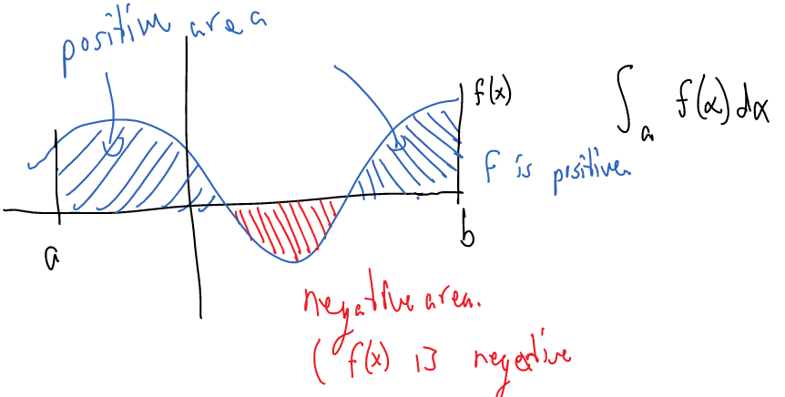
When we say “area under the curve” we mean the signed area, meaning that regions above the $x$ axis have positive area and regions below the $x$ axis have negative area.

Example:

If we have the following curve with the following areas:

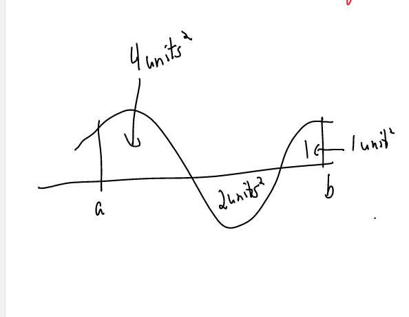
On the interval from $a$ to $b$, there are two regions above the $x$ axis with areas 4 and 1; there is one region below the $x$ axis with area 2. Find $\int_a^b f(x) \, dx$

Solution: Add the signed areas: $\int_a^b f(x)\, dx = 4 + (-2) + 1 = 3$.

Properties of the integral

Here are many, many properties of the integral. Do you need to memorize them? Oh yes, definitely! But don’t worry, you don’t have to commit them all to memory right now. We’ll be using them frequently through the rest of calculus 1 - 3. Just be familiar with this list.

• $\displaystyle \int_a^b f(x)\, dx = - \int_b^a f(x) \, dx$
• $\displaystyle \int_a^a f(x)\, dx = 0$
• $\displaystyle \int_a^b c \, dx = c (b-a)$ where $c$ is a constant
• $\displaystyle \int_a^b c f(x)\, dx = c \int_a^b f(x)\, dx$
• $\displaystyle \int_a^b f(x) \pm g(x) \, dx = c\int_a^b f(x)\, dx \pm \int_a^b g(x)\, dx$
• $\displaystyle \int_a^b f(x)\, dx = \int_a^c f(x)\, dx + \int_c^b f(x)\, dx$ if $a < c < b$.
• If $\displaystyle f(x) \ge 0$ for $a \le x \le b$, then $\displaystyle \int_a^b f(x)\, dx \ge 0$.
• If $\displaystyle f(x) \ge g(x)$ for $a \le x \le b$, then $\displaystyle \int_a^b f(x)\, dx \ge \int_a^b g(x)\, dx$.

Example

Evaluate the following integral by using properties above and interpreting the integral as area:

$$ \int_0^5 x + 1 \, dx $$

Example

Evaluate the following integral by using properties above and interpreting the integral as area:

$$ \int_{-5}^5 x - \sqrt{25-x^2} \, dx $$

Example

Evaluate the following integrals by using properties above and interpreting the integral as area. The graph of $y=f(x)$ is shown below:

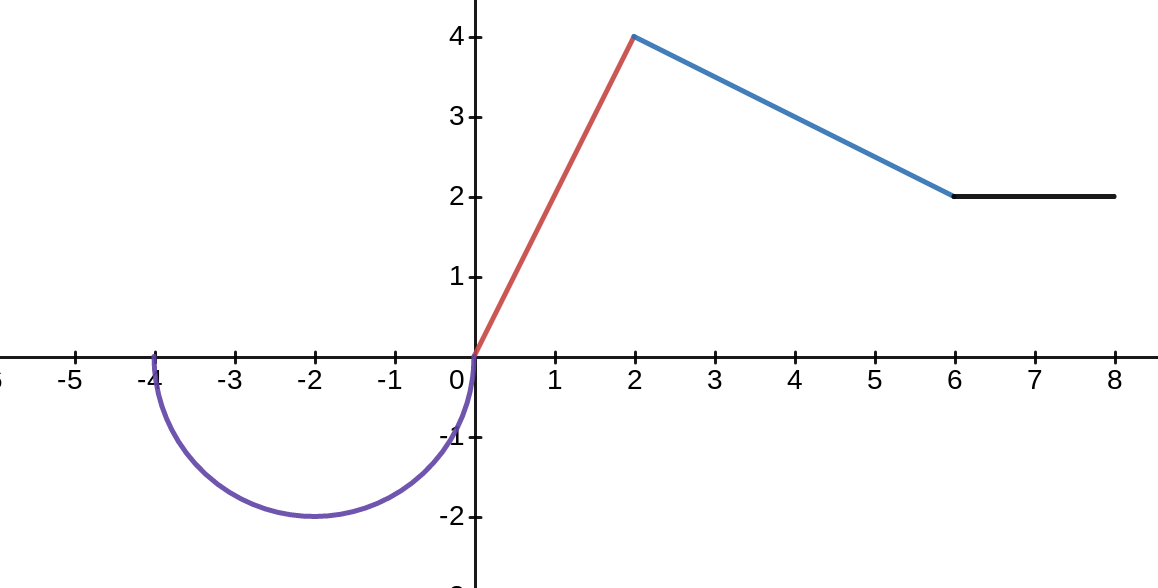
1. $\displaystyle \int_{-2}^0 f(x)\, dx$
2. $\displaystyle \int_{0}^6 f(x)\, dx$
3. $\displaystyle \int_{-4}^8 f(x)\, dx$

Numerical Approximations of Integration:

Approximation Spreadsheet

Here’s a link to the spreadsheet I will be using during class.

###NOAA Weather Data Here’s a link to NOAA Weather Data for the Little Arkansas River floodway (closest weather station I could find to Wichita State)