1.5 The Limit

This is section 1.5

The question:

What happens to the $y$-values of a function as the $x$-values get closer to a particular value?

Limits: An informal definition

We write $\displaystyle \lim_{x \to a} f(x) = L$ and say “the limit of $f(x)$, as $x$ approaches $a$, is $L$” if we can make the values of $f(x)$ arbitrarily close to $L$ (as close to $L$ as we want) by making the values of $x$ sufficiently close to $a$ but not equal to $a$.

i.e. “You want this part machined within 0.001mm error tolerance (y-values)? I can adjust my tools (x-values) to do that!”

Example

Guess the value of $\displaystyle \lim_{x\to 1} \frac{x-1}{x^2 -1}$

note: you can’t just plug in $1$ because that function isn’t defined there.

Example

Take a moment guess the value of $\displaystyle \lim_{x\to 0} \dfrac{\sin x}{x}$.

Note: In calculus, we’re nearly always using radians, so these $x$ values are radians. If you’re using Google Sheets, the =SIN function automatically uses radians. If you’re using a calculator (or another tool) make sure you’re in radian mode.

One-sided limits

Definition:

We write $$ \lim_{x\to a^-} f(x) = L $$ and say the limit of $f(x)$ as $x$ approaches $a$ from the left is equal to $L$ if we can make the values of $f(x)$ arbitrarily close to $L$ (as close to $L$ as we want) by making the values of $x$ sufficiently close to $a$ but not equal to $a$.

Similarly, we define $$ \lim_{x\to a^+} f(x) = L $$ to be the right-hand limit.

Connection to total limit

We say that: $$ \lim_{x \to a} f(x) = L \text{ if and only if } \lim_{x\to a^-} f(x) = L \text{ and } \lim_{x\to a^+} f(x) = L $$

Some visual examples

Here’s a Geogebra applet that demonstrates visually different one-sided and two-sided limits compared to the total limit. Click ‘animate’ next to each limit and watch as the $y$-values as the $x$-values get close to the desired number.

Be sure to adjust the slider that says Example = # because that shows three different limit examples.

https://www.geogebra.org/m/AKbRXpJJ

Note that, from the Geogebra applet:

1. On example 1, the left and write limits are the same, so $\lim_{x\to -3} f(x) = 3$, even though the function’s value is -1 there, and
2. On example 3, because the left and right limits aren’t the same, we say $\lim_{x\to 2} f(x)$ does not exist and often write DNE.

Infinite Limits

Example

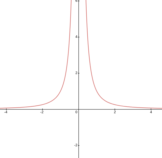
Consider $\displaystyle \lim_{x\to 0} \frac1{x^2}$.

That graph obviously looks like this:

Looking at the left and right limits, we have:

$\lim_{x\to 0^-} \frac{1}{x^2} = \infty$ and $\lim_{x\to 0^+} \frac{1}{x^2} = \infty$

Because both sides tend to the same value, we say that limit $\displaystyle \lim_{x\to \infty} \frac{1}{x^2} = \infty$. The limit does not exist and $\infty$ is not a number, but because the left and right limits agree on the same value, we write the special value this way.

Compare to the next example

Example

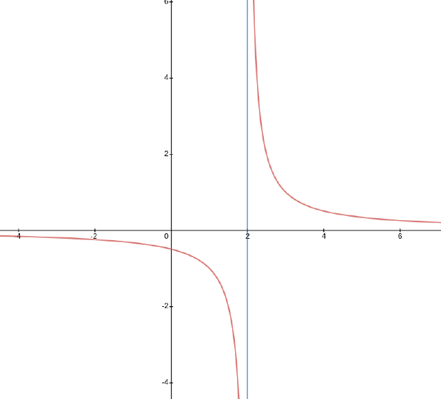
Consider the limit $\displaystyle \lim_{x\to 2} \dfrac{1}{x - 2}$.

The graph is this one:

This time, my one-sided limits are as follows:

$\displaystyle \lim_{x\to 2^-} \frac{1}{x-2} = -\infty$ while $\displaystyle \lim_{x\to 2^+} \frac{1}{x-2} = \infty$.

… in this case, the limits don’t agree, so we still say that the limit doesn’t exist but we write $\displaystyle \lim_{x\to 2} \frac{1}{x-2} = \text{DNE}$.

Visually exploring vertical asymptotes

If you want to play with another geogebra applet, this one explores vertical asymptotes as limits. Here, you’ll click the points and move them left and right. Watch as the x-values get close to the location of the asymptote and see the y-values head up to infinity or down to negative infinity. These are infinite limits from the left and right!

https://www.geogebra.org/m/PSrua4JF

Now practice!

Head over to WebAssign and work on section 1.5. If you have questions, let me know!

This is section 1.6

The limit laws

Suppose $c$ is a constant and the limits: $$ \lim_{x\to a} f(x) \text{ and } \lim_{x\to a} g(x) $$ exist and are finite. Then:

1. $\displaystyle \lim_{x\to a} [ f(x) + g(x) ] = \lim_{x\to a} f(x) + \lim_{x \to a} g(x)$
2. $\displaystyle \lim_{x\to a} [ f(x) - g(x) ] = \lim_{x\to a} f(x) - \lim_{x \to a} g(x)$
3. $\displaystyle \lim_{x\to a} [ cf(x) ] = c \cdot \lim_{x\to a} f(x)$
4. $\displaystyle \lim_{x\to a} [ f(x) g(x) ] = \lim_{x\to a} f(x) \cdot \lim_{x \to a} g(x)$
5. $\displaystyle \lim_{x\to a} \frac{f(x)}{g(x)} = \frac{\lim_{x\to a} f(x)}{\lim_{x \to a} g(x)}$ if $\lim_{x\to a} g(x) \ne 0$.
6. $\displaystyle \lim_{x\to a} [ f(x) ]^n = [\lim_{x\to a} f(x)]^n$ if $n$ is a number

Examples

Below I work many examples in the video

Caution!

The limit laws only work if the limit exists and is finite! For example, we know $$ \lim_{x\to 0} \frac{1}{x^2} = 0 \text{ and } \lim_{x\to 0} \frac{1}{x^4} = 0 $$ but … $$ \lim_{x\to 0} \frac{1/x^2}{1/x^4} = \lim_{x\to 0} \frac{x^4}{x^2} = \lim_{x\to 0} x^2 = 0 $$

The Squeeze Theorem

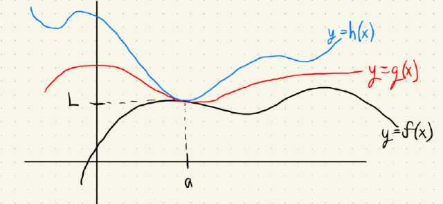
If $f(x) \le g(x) \le h(x)$ when $x$ is near $a$ $$ \lim_{x\to a} f(x) = \lim_{x\to a} h(x) = L $$ then $\displaystyle \lim_{x\to a} g(x) = L$.

Here’s an illustration of the red function $g(x)$ being squeezed between the upper blue function $h(x)$ and the black function $f(x)$ from below at the point $x=a$.

Example

Show that $\displaystyle \lim_{x\to 0} x^2 \sin\left( \frac{1}{x} \right) = 0$

Now practice!

Head over to WebAssign and work on section 1.6. If you have questions, let’s talk about them!